Time Series II + Panel

Paulo Fagandini

Nova SBE

Exercises

https://moodle.novasbe.pt/mod/folder/view.php?id=4021

Exercise 11.5

Using US data for hte period 1960-2005, the following regression of wages on productivty in the business sector was estimated:

\[\widehat{\ln Comp_t}=\underset{(0.0547)}{1.6067} + \underset{(0.0124)}{0.6522} \ln Prod_t\]

Exercise 11.5-a

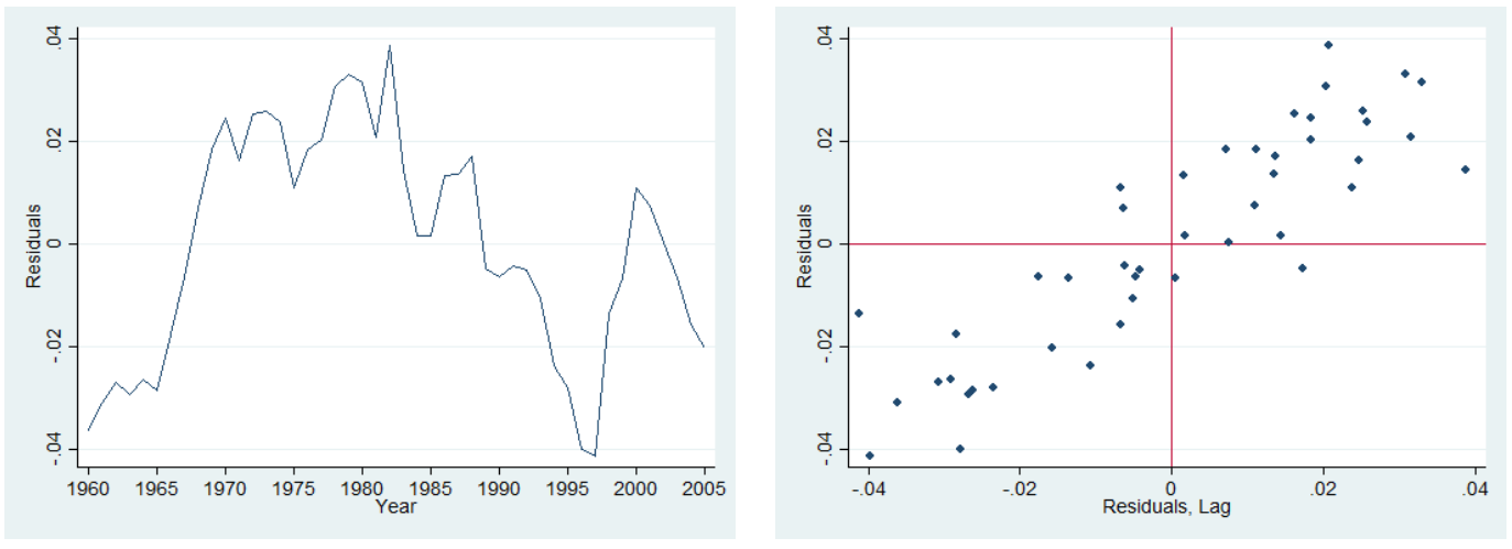
Below you have the plot of the residuals from the regression along time (left) and the plot of the residuals against their first lag (right). What can you conclude regarding serial correlation?

Plot 1: the residuals are systematically positive/negative Plot 2: The residuasl and their lads are (strongly) positively correlated There is evidence of serial correlation (at least of order 1)

Exercise 11.5-b

The Durbin-Watson (DW) for the above regression is 0.218. What do you conclude? State the null and the appropriate alternative for this test. What are the critical values that you consider for this test? Why?

Under the null and alternative hypotheses: \(H_0=\rho=0\) and \(H_a: \rho >0\) In the table of the DW we have two values \(d_L\) and \(d_u\). In the exercise \(n=46\), \(k=1\), \(\alpha=5%\): \(d_L=1.48\) and \(d_U=1.58\).

Since \(DW=0.218 < d_L\) we reject the \(H_0\) and there is evidence of \(AR(1)\) serial correlation.

Exercise 11.5-c

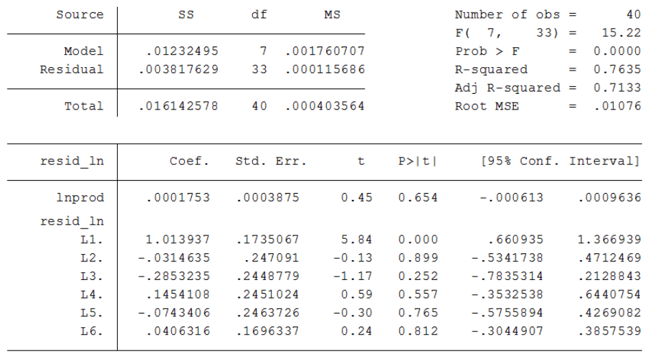
A higher order of autocorrelation (6) was tested using the Breusch-Godfrey tets. What do you conclude from the output of this test, provided below?

BG of higher order of serial correlation (order 6). Including the independent variables (\(lnprod\)) makes the test valid with or without strict exogeneity.

Note \(LN=(n-q)R^2\). \(n-q\) is the number of observations left when taking into account the obs lost due to the lags.

\(LM=(46-6)\times 0.7635=30.54>12.59\) (critical value from \(\chi^2_6\) at 5%)

Reject the null of no serial correlation! (Only \(\hat{u}_{t-1}\) individually significant, suggest \(AR(1)\))

Exercise 4.5-d

Suspecting model misspecification, a trend was added to the initial model. Considering the reported estimates below, what do you conclude? Is there still eevidence for autocorrelation?

\[\widehat{\ln Comp_t}=\underset{(0.307)}{0.121}-\underset{(0.002)}{0.008}t+\underset{(0.0776)}{1.0283} \ln Prod_t\]

With \(DW=0.45\)

In the exercise \(n=46\), \(k=2\), \(\alpha=5%\), \(d_L=1.43\), \(d_U=1.62\). Since \(DW<d_L\) we reject the \(H_0\) and there is still evidence of \(AR(1)\) serial autocorrelation.

Exercise 4.5-e

Three alternatives were cosnidered in order to corect for autocorrelation:

1. Initial model in first-differences \(\widehat{\Delta \ln Comp_t}=\underset{(0.057)}{0.654}\Delta \ln Prod_t\) with \(DW=1.74\)
2. Model with trend in first-differences \(\widehat{\Delta \ln Comp_t} = \underset{(0.003)}{0.001}+\underset{(0.109)}{0.619}\Delta\ln Prod_t\) with \(DW=1.71\).
3. Quasi-differenced initial model (Cochrane-Orcutt esitmation): \[\widehat{\ln Comp_t}=\underset{(0.192)}{1.955}+\underset{(0.042)}{0.577} \ln Prod_t^*\] with \(\hat{\rho}=0.869\), \(DW=1.70\)

Is the problem of autocorrelation solved?

In the exercise \(n=45\), \(k=1\), \(\alpha=5%\), \(d_U=1.48\), \(d_L=1.57\)

Since for all alternatives \(4-d_U>DW>d_U\) we fail to reject the \(H_0\) and there is not enough evidence to reject the absence of autocorrelation.

Exercise 4.5-f

Consider the following heteroskedasticity test for the initial model:

\[\hat{u}_t^2=\underset{(23.64)}{94.27}-\underset{(0.514)}{1.836}\widehat{\ln y_t} + \underset{(0.003)}{0.009}\widehat{\ln y_t}^2\] with \(n=46\) and \(R^2=0.296\)

What do you conclude? Is there a solution for both serial correlation and heteroskedasticity?

\(LM=46\times 0.296=13.754>5.99\) (critical value from \(\chi_2^2\) at \(5%\))

There is evidence of heteroskedasticity

Newey-West s.e. account for both, heteroskedasticity and serial correlation!

Exercise 4.5-g

Consider the following estimates for the initial model with \(Newey-West\) standard errors. How do they compare with theusual standard errors?

\[\widehat{\ln Comp_t}=\underset{(0.079)^*}{1.607}+\underset{(0.018)^*}{0.652}\ln Prod_t\]

They are higher than usual standard errors. Still, the coefficient is statisticall significant. \(t=0.652/0.018=36\).

Exercise 12.1

You are provided with a panel dataset of 400 firms observed over 5 years (from 2015 to 2019). The dataset includes the following variables:

• irm id: Firm identifier.
• year: Year of observation.
• R&D expense: Annual R&D expenditure (in millions of dollars).
• profit: Annual profit before tax (in millions of dollars).
• capital: Total capital stock (in millions of dollars).
• industry: Categorical variable indicating the industry sector (values 1 to 8).
• age: Age of the firm (in years).
• CEO tenure: Tenure of the CEO (in years).

Exercise 12.1

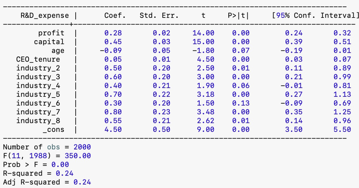
You are interested in studying the determinants of R&D expenditure, focusing on how profit, capital stock, and industry sector influence a firm’s investment in R&D. Below are outputs from statistical software for three models estimated using this dataset.

Pooled

Exercise 12.1

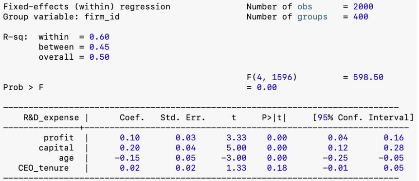
You are interested in studying the determinants of R&D expenditure, focusing on how profit, capital stock, and industry sector influence a firm’s investment in R&D. Below are outputs from statistical software for three models estimated using this dataset.

Fixed Effects

Exercise 12.1-a

Explain the main differences between the pooled OLS model, the fixed effects model, and the random effects model in the context of this study on R&D expenditure. Discuss the assumptions underlying each model, especially regarding the inclusion of the industry variable.

Pooled OLS Model: * Treats the panel data as a large cross-sectional dataset, ignoring the panel structure (time and individual dimensions). * Includes all variables, including time-invariant variables like industry, as regressors. * Assumes there are no omitted variables that vary across firms or over time and are correlated with the regressors. * Assumes exogeneity: Regressors, including industry, are uncorrelated with the error term.

Fixed Effects: * Controls for unobserved time-invariant heterogeneity by allowing each firm to have its own intercept (firm-specific effects). * Focuses on within-firm variations over time. * Time-invariant variables like industry are omitted because their effects are absorbed by the fixed effects. * Assumes unobserved firm-specific effects are constant over time. * Allows for correlation between unobserved effects and the regressors. * Provides consistent estimates even when unobserved firm characteristics are correlated with the regressors. * Cannot estimate the effect of time-invariant variables like industry.

Exercise 12.1-b

Based on the outputs provided, interpret the estimated coefficients for profit and capital in all three models. Discuss why the estimates for these variables might differ among the pooled OLS, fixed effects, and random effects models.

Pooled OLS Model: * profit: An increase of $1 million in profit is associated with an increase of $0.28 million in R&D expenditure, ceteris paribus. * capital: An increase of $1 million in capital stack is associated with an increase of $0.45 million in R&D expenditure, ceteris paribus.

Fixed Effects: * profit: An increase of $1 million in profit is associated with an increase of $0.1 million in R&D expenditure, ceteris paribus. * capital: An increase of $1 million in capital stack is associated with an increase of $0.2 million in R&D expenditure, ceteris paribus.

The Pooled OLS coefficients for profit and capital are higher than those in the FE model. This suggests that unobserved firm-specific characteristics correlated with profit and capital may inflate the estimated effects in Pooled OLS model. By accounting for time-invariant firm characteristics, the FE model reduces potential bias, resulting in lower (and potentially more accurate) estimates.

Exercise 12.1-c

The fixed effects model does not include the industry variables in the output. Explain why this occurs and discuss the implications for interpreting the effect of industry sector on R&D expenditure.

The industry variables are time-invariant for each firm (firms do not change industries over time). In the FE model, time-invariant dummies are perfectly collinear with the firm-specific fixed effects. This means FE cannot estimate the coefficients of industry as the effect of industry on R&D expenditure (together with all other time-invariant characteristics) is absorbed into the fixed effects

Exercise 12.1-d

Explain why the constant term is omitted in the fixed effects model. How are the firm-specific intercepts and time-invariant variables handled in this model?

The Fixed Effects model includes firm-specific intercepts (fixed effects) for each firm. Including a general constant term would cause perfect multicollinearity since the sum of the fixed effects and the constant would not be identifiable. Each firm has its own intercept, capturing all time-invariant characteristics unique to that firm.

Exercise 12.1-e

Considering that CEO tenure may change over time for each firm, discuss its estimated effect in each model. Based on the outputs, does CEO tenure have a significant impact on R&D expenditure? How might the interpretation differ across models?

Pooled OLS Model: * Coefficient(0.05), p-value = 0.01: CEO tenure is statistically significant. A one-year increase in CEO tenure is associated with an increase of $0.05 million in R&D expenditure.

Fixed Effects: * Coefficient(0.02), p-value = 0.18: CEO tenure is not statistically significant at any reasonable level. Within a firm, changes in CEO tenure over time do not significantly affect R&D expenditure.

In Pooled OLS, unobserved firm-specific characteristics correlated with CEO tenure may inflate its estimated effect. The FE model controls for these unobserved characteristics, re- ducing both the coefficient and its significance. This means the impact from CEO tenure may actually be driven by between-firm variation. Within-firm changes in CEO tenure may not significantly impact R&D expenditure.

Exercise 12.1-f

Discuss how unobserved heterogeneity might affect the estimates in the pooled OLS and random effects models, particularly regarding the industry variable. Why might the fixed effects model provide more reliable estimates in the presence of unobserved heterogeneity?

Unobserved firm-specific characteristics (e.g., management quality, innovation culture) that are time-invariant and affect R&D expenditure may be correlated with regressors like profit, capital, and industry. Pooled OLS does not adequately control for unobserved heterogeneity if it is correlated with the regressors. This can lead to biased and inconsistent estimates.

Fixed Effects controls for all time-invariant unobserved heterogeneity by using within-firm variation. This provides consistent estimates even when unobserved firm-specific effects are correlated with the regressors.

Regarding industry variables: In Pooled OLS model, the effect of industry may capture both observed and unobserved industry characteristics. If unobserved heterogeneity is present, the estimates for industry may still be biased in these models.